Design space exploration

This guide provides an overview and brief instructions on using Design space exploration blocks to solve design space exploration problems by leveraging design of experiment and optimization techniques.

Design space exploration is a beta block

The Design space exploration block is in beta. Future pSeven Enterprise updates will keep compatibility with the current version of the block, but this beta version may still have some features missing or not yet working as intended.

The Design space exploration block can generate design of experiment samples with specific properties, collect response samples from other blocks evaluating those designs, and solve optimization problems. It also provides advanced methods such as adaptive design generation, response function contour restoration, gradient-based and surrogate-based optimization.

This block employs a task-based approach: its configuration focuses on defining the design space (variables, responses, and their properties) and design goals which can be set individually for each response. To aid you in configuration, the block supports the SmartSelection technology which recommends the method to use based on your design space definition. This approach allows you to easily switch between tasks and even to combine several methods in a single study.

Getting started

The Design space exploration block solves a variety of design problems related to studying the behavior of some computational model. You can begin your study with generating a design of experiment sample with specific properties, then add functional constraints, generate an adaptive design of experiment optimized for a more accurate representation of the model responses, or run optimization. All these tasks use the same definitions of variables and responses, so it is easy to switch between them without reconfiguring the block.

There are two typical setups for Design space exploration block in a workflow:

1. Sample generator - setup where you describe only design variables and their properties.
2. Blackbox driver - setup where you describe design variables and responses from the model under study. This setup requires connecting the Design space exploration block to other blocks that evaluate model responses - so called blackboxes.

With the sample generator setup, the block receives all required information from its settings - properties of design variables and technique options you specify. Also, it can receive an optional initial sample, which in this case is updated with newly generated design points.

flowchart TB
  classDef dashed stroke-dasharray: 3 5;
  settings[\ /]:::dashed
  insample[\ /]:::dashed
  dse(Design space exploration)
  outsample[\ /]
  settings .->|Settings| dse
  insample .->|Initial sample| dse
  dse -->|Generated sample| outsample

The sample generator setup is used for such tasks as:

• Generating a space-filling design of experiment sample within the variables' bounds. The space-filling properties of this sample depend on the generation technique you select.
• Updating an existing design of experiment, which is sent to the block as the initial sample. By default, the block just adds points from the initial sample to its output sample - that is, the initial sample data is not used in the generation process. However, some techniques can be configured to "continue" generating the initial sample, preserving its properties.

With the blackbox driver setup, the Design space exploration block becomes a tool for performing computational experiments according to the generated design. This setup adds responses to the block's settings. Together, the variables and responses describe the inputs and outputs of some computational model. However, the Design space exploration block does not define or calculate this model: you have to create one or more blackboxes - blocks that evaluate model outputs - and connect them to the Design space exploration block. The optional initial sample in this case can contain values of responses in addition to values of variables.

flowchart TB
  classDef dashed stroke-dasharray: 3 5;
  settings[\ /]:::dashed    
  insample[\ /]:::dashed
  dse(Design space exploration)
  blackbox(Blackbox)
  results[\ /]
  settings .->|Settings| dse
  insample .->|Initial sample| dse
  dse -->|Variables| blackbox
  blackbox -->|Responses| dse
  dse -->|Results| results

When running with this setup, the Design space exploration block sends values of design variables to the connected blackboxes and receives values of responses. A blackbox can be a Composite block containing some computational chain or a set of blocks, which calculate different outputs of the model. The final results contain all data exchanged with the model - both the design of experiment (values of variables) and the outcome (response values).

The blackbox driver setup is used for such tasks as:

• Solving optimization problems.
• Generating a space-filling design of experiment sample subject to functional constraints.
• Generating a design of experiment sample and evaluating model responses for this sample.
• Evaluating model responses for an existing input sample, without generating new points.

Configuration basics

The first and the most important step when configuring the Design space exploration block is defining variables and responses. Based on these definitions, the block automatically selects the appropriate technique (SmartSelection mode). You can further tune this technique manually, using the automatically selected settings as initial recommendations.

Basic configuration dialog elements:

• The Variables pane and Responses pane serve to define the variables and responses.
• The toggle turns SmartSelection on or off.
• The "Technique" field displays the currently selected study technique and allows you to choose a different technique.
• The "Options" field displays the current non-default option settings for the selected study technique. Use the button to access all option settings.
• The settings in the "Exploration budget" and "Study target" fields above the Responses pane determine the response evaluation limit along with the study target for the Adaptive design technique (see later in this section).
• The "Hints" field above the Responses pane displays the currently selected general hints that affect the study technique settings in SmartSelection mode (see later in this section). You can add or remove hints from this field.
• Use the "Run options" button to access a number of settings that control the operation of the block in the workflow (see Run options).
• Use the "Ports and parameters" button to view or change port settings and to specify which ports serve as workflow parameters (see Ports and parameters).

To change study technique options, first disable SmartSelection by using the button. Then, you can select the desired technique from the "Technique" drop-down, and configure technique options. The button opens the technique configuration dialog with a list of options; for each option, you can view its description in a tooltip.

Depending upon the selected study technique, the "Exploration budget" field setting determines the maximum number of designs to evaluate or the number of points in the design of experiment sample to generate. This setting is optional: with the Auto value (default), the appropriate budget is set automatically, considering the number of variables and responses, the study technique, its options, and other block settings. The "Exploration budget" field provides a tooltip that explains the effect of the current setting on the block configuration.

In the case of the Adaptive design technique, you can use the "Study target" setting to specify the desired number of feasible designs. This setting is optional, and it has the following effect when using the Adaptive design technique:

• If you do not set the exploration budget and do not specify the study target, the block selects them automatically, depending on the design space dimension and the value of the technique's Accelerator option. Since each of these parameters is set to a certain finite value, the generation ends as soon as the block finds an appropriate number of feasible designs, or when the automatically selected budget is exhausted, whichever occurs first.
• If you set a certain exploration budget without specifying the study target, the block generates as many feasible designs as possible within that budget. The generation ends as soon as the exploration budget is exhausted.
• If you specify a certain study target without setting the exploration budget, the block generates new designs until it finds the specified number of feasible designs. This may require significantly more response evaluations than the study target setting specifies, depending upon the response behavior.
• If you set both the exploration budget and study target, the block aims to generate the specified number of feasible designs within the given exploration budget. The generation ends as soon as the block finds the target number of feasible designs, or when the budget is exhausted, whichever occurs first. If the budget is not large enough, the block may find fewer feasible designs than the study target.

The block automatically validates its configuration and notifies you if any issues are found. The button toggles the validation issues pane, where you can view the details.

• A warning message indicates that the block can start but an error may occur during the workflow run, or you can encounter unexpected results.
• An error message indicates that the block cannot start. A workflow with this block will not start either.

Important

Warnings may provide valuable information and configuration hints. A good practice is to review all warnings issued by the block and fix them before running the workflow, unless you are sure that the behavior described in a warning is acceptable for your task.

There are some general configuration hints that you can use to provide the block with additional information about the task. In the "Hints" field above the Responses pane:

• Add the Noisy responses hint if the initial sample data or some response evaluations contain noise.
• Add the Cheap responses hint if all responses are computationally cheap (fast to evaluate).

In SmartSelection mode, the block takes these hints into account to adjust the recommended settings.

Variables

Design variables are a mandatory part of the block configuration. The block configuration dialog provides the Variables pane for managing variables. In this pane, you can add or remove variables, as well as view or change their properties.

Adding a variable automatically creates the result output ports specific to that variable, in addition to the common result outputs. If any responses are already defined in the block's configuration, it also creates the request port to output values of that variable for blackbox evaluations (see Blackbox ports and connections). In the Ports and parameters dialog, you can enable additional result ports and special input ports to set or change the properties of the variable and to receive initial sample data, see Ports and parameters and Initial samples for further details.

The main properties of a variable:

• Name - Identifies the variable and related ports.
• Type - The variable can be continuous (default), discrete, stepped, or categorical. The block treats each of these types in a special way.
• Size - The number of components in the variable (its dimension). You can add an input port that sets this property.
• Lower bound - The minimum allowed value for a continuous or a stepped variable. Ignored if the variable is discrete, categorical, or constant. You can add an input port that sets this property.
• Upper bound - The maximum allowed value for a continuous or a stepped variable. Ignored if the variable is discrete, categorical, or constant. You can add an input port that sets this property.
• Levels - Predefined values for discrete and categorical variables. Ignored for continuous variables and constants. You can add an input port that sets this property.

The additional properties, set by variable hints:

• Constant - A variable of any type can be set to constant, which allows you to freeze a variable - essentially, exclude it from consideration without deleting it. You can add an input port that sets this hint. The "Constant" hint only sets a variable to constant (freezes or unfreezes a variable), and requires the "Value" hint which specifies the fixed value.
• Initial guess - Sets the initial guess value in optimization. Ignored by design of experiment techniques; also ignored for constant variables (see the description of the "Value" hint). You can add an input port that sets this hint.
• Resolution - Specifies the minimum significant change of a continuous variable. Ignored for variables of other types.
• Step - This hint is required for a stepped variable and sets its step. Ignored for variables of other types.
• Value - The value for the constant variable. Ignored if the "Constant" hint is not set. You can add an input port that sets this hint.

For a detailed description of the properties and hints listed above, see Variable properties and Variable hints.

Generally, you are required to set those properties that are not ignored for the selected type of the variable. For example, the size of the variable must always be set, bounds are required for continuous variables, and so on. You can also set ignored properties - their values are saved in the block's configuration, so you can use them later. Values of ignored properties are grayed out in the Variables pane.

Variable properties

The main properties of the variable are as follows:

• Name

  The name identifies the variable, and is part of the names of its ports. The name is assigned to the variable when it is created, you can change the name in the Variables pane. When renaming a variable, the name of each of its ports changes accordingly.

  Each variable must have a unique name among all variables and responses within the block configuration, and it must contain only allowed characters. The following characters are not allowed in variable names: . < > : " / \ | ? *. Variable names are checked in the block configuration dialog; if you try to give a variable a name with characters that are not allowed, the dialog displays an appropriate message.

• Type

  A variable can be continuous (default type), discrete, stepped, or categorical:

  • Continuous - generic variable that may take any numeric value within the design bounds. The bounds ("Lower bound" and "Upper bound" properties) are required for continuous variables.
  • Stepped - a variable that may take numeric values distributed evenly within bounds, from lower to upper, at regular intervals - steps. A stepped variable requires bounds to be specified along with the "Step" hint to set the step size.
  • Discrete - a variable with a finite set of allowed numeric values ("Levels" property). Levels are required for discrete variables, and must be numeric; the bounds are ignored. Specifically, you can use this type to describe an integer variable.
  • Categorical - a variable with a finite set of allowed levels that can be numeric or string values. Categorical variables require levels to be specified, and disregard the bound settings.

  Internally, a stepped variable is similar to a continuous one, but with values adjusted to the regular grid defined by the variable's bounds and step. A discrete variable may have arbitrary levels, although it is recommended to use this type only for true integer variables, or variables that cannot be defined as stepped.

  Discrete and categorical variables are processed differently by the block's design generation and optimization algorithms:

  • Values of a discrete variable can be compared numerically (less, greater, or equal). They can be ordered and used in arithmetic operations.
  • Values of a categorical variable can be compared only for equality, even if all of them are numerical.

  For more details on configuring variables of different types, see Variable types.

• Size

  This property specifies the number of components in the variable, that is, the dimension of the variable. For example, if you do not want to create multiple variables of the same type, you can add a single multi-dimensional variable instead. Components of this variable can have different bounds or sets of levels.

  The "Size" property affects the following:

  • The syntax of the following properties and hints: "Lower bound", "Upper bound", "Levels", "Initial guess", "Resolution", "Step", and "Value". See Variable types for details.
  • The number of columns corresponding to this variable in the initial sample tables. See Initial samples for details.
  • The number of the corresponding columns in the result tables. See Block operation results for details.

  • The type of variable values the block sends to blackboxes for evaluation - a numeric scalar if "Size" is 1, or a numeric vector if "Size" is greater than one. In the latter case, the number of vector components is equal to the "Size" property value.

    If batch mode is enabled (see Batch mode), then, depending upon the "Size" property of the variable, its value is a one-dimensional array of scalar or vector values, with the number of array elements determined by the Maximum batch size option setting.

    See Blackboxes for details.

  Note that you can use a special input port to set the "Size" property (for details, see Ports and parameters). Specifically, this enables you to create variables of varying dimension that can quickly be changed by using workflow parameters.

• Lower bound, Upper bound

  The lower and upper bounds specify, respectively, the minimum and maximum allowed values for a variable. This property is required for continuous and stepped variables (see the "Type" property description). Also, the Gradient-based optimization and Surrogate-based optimization techniques require that the range between bounds be at least $10^{-6}$. Constant, discrete, and categorical variables ignore bound settings and do not validate them.

  The value of a bound can be a number or a vector:

  • A number value sets the same bound for all components of the variable. Such a setting is normally used for one-dimensional variables (those of size 1); however, it can also be used for multi-dimensional variables.
  • A vector value sets an individual bound for each component. The number of vector components must be equal to the value of the variable's "Size" property.

  For syntax examples, see Variable types.

  Note that you can set bounds by using special input ports (for details, see Ports and parameters).

• Levels

  In the case of a discrete or categorical variable (see the "Type" property description), you must define a finite set of its allowed values called levels. Constant variables of any type, continuous and stepped variables ignore this property and do not validate it.

  The value of the "Levels" property can be a single vector or a list of vectors:

  • A single vector specifies the same set of levels for each component of the variable. Such a setting is normally used for one-dimensional variables (those of size 1); however, it can also be used for multi-dimensional variables.
  • A list of vectors specifies an individual set of levels for each component of the variable. The number of list elements (vectors) must be equal to the variable's "Size" property.

  For syntax examples, see Variable types.

  Every vector representing a set of levels (for a variable or its component) must have at least 2 components, since a discrete or categorical variable with 1 level is just a constant. Also, for discrete variables the type of the vector implicitly determines whether the values of the variable values are floating-point numbers or integers.

  Note that you can use a special input port to set the "Levels" property (for details, see Ports and parameters).

Variable hints

The following hints are used to manage additional properties of the variable:

• Constant

  A constant variable has a fixed value defined by the "Value" hint. This value is the same in all generated designs. A constant variable generates a constant column (columns, if its "Size" is greater than 1) in the result tables. One exceptional case is when you add an initial sample for a constant variable: the values in the initial sample can be non-constant and are not required to be equal to the variable's "Value" hint. If the initial sample is added to results, you can encounter a non-constant column for a constant variable (for more details, see Initial samples).

  This hint is mostly intended as a means to temporarily exclude a variable from consideration while keeping the variable's settings and the links connected to the related ports.

  You can also switch a variable to constant when you want to try some value out of bounds or to give some stepped variable a value that does not match any step. This is possible because constant variables ignore the bounds, levels, and step settings, and do not validate them, so you do not need to change those settings.

  This hint only switches the variable to constant and additionally requires the "Value" hint to specify the constant value for the variable. Note that you can use special input ports to make the variable a constant and set the constant value (for details, see Ports and parameters).

• Initial guess

  This hint specifies an initial guess value (the starting point) for optimization techniques. Specifically, when using the Gradient-based optimization technique, it is highly advisable to set a certain initial guess for all variables. Globalized optimization methods also use this value - for example, as one of the multi-start points. The initial guess settings are ignored by all techniques except Gradient-based optimization and Surrogate-based optimization, and are always ignored for constant variables (to set the value of a constant, use the "Value" hint).

  The following requirements apply to the initial guess setting:

  • For a continuous or a stepped variable, the initial guess must be within the variable's bounds.
  • For a stepped variable, the initial guess must also be a valid value according to the step size (the "Step" property).
  • For a discrete or categorical variable, the initial guess must be a valid value according to the "Levels" property.

  The "Initial guess" value can be a scalar or a vector:

  • A scalar value sets the same initial guess for all components of the variable. Such a setting is normally used for one-dimensional variables (those of size 1); however, it can also be used for multi-dimensional variables.
  • A vector value sets a specific initial guess for each component. The number of vector components must be equal to the value of the variable's "Size" property.

  For syntax examples, see Variable types.

  Note that you can set the initial guess by using a special input port (for details, see Ports and parameters).

• Resolution

  This optional hint for a continuous variable specifies the minimum significant change of the variable. For example, if the variable is bound to the range $[1000.0, 5000.0]$, its changes less than 1 most likely do not change responses noticeably, in which case you can set the resolution to 1.0.

  In optimization tasks, it is recommended to set the "Resolution" hint for all continuous variables, as this enables the block to adjust precision of optimization algorithms accordingly, and often improves performance. The "Resolution" value should be based on the real, practical precision of a design variable. The minimum valid value is $10^{-8}$. The maximum valid value is $0.1 \cdot r$, where $r$ is the range between the bounds - although in practice such resolution is too coarse and is not recommended.

  The "Resolution" value can be a scalar or a vector:

  • A scalar value sets the same resolution for all components of the variable. Such a setting is normally used for one-dimensional variables (those of size 1); however, it can also be used for multi-dimensional variables.
  • A vector value sets a specific resolution for each component. The number of vector components must be equal to the value of the variable's "Size" property.

  For syntax examples, see Variable types.

  This hint is ignored by all types of variables except continuous, and is currently ignored by the design of experiment generation techniques.

• Step

  In the case of a step variable, this hint is required to set the size of the variable's step. Note that the step size $s$ should be relatively small compared to the range between bounds $r$: the greatest valid step size is $s_{\rm{max}} = 0.1 \cdot r$, but in practice it is recommended to use steps with size $s \le 0.01 \cdot r$. In addition, the range between the bounds of the variable must contain an integer number of steps, in other words, $r$ must be a multiple of the step size $s$.

  So, the step size $s$ must meet the following requirements:

  • $s \ge 10^{-8}$, but note that $s$ is also validated against the bounds range $r$.
  • $s \ge 10^{-4} \cdot r$, where $r$ is the range between the variable's bounds.
  • $s \le 0.1 \cdot r$, but note that it is recommended to have $s \le 0.01 \cdot r$.
  • $s \cdot k = r$, where $k$ is some integer - the range must be a multiple of the step size.

  The "Step" value can be a scalar or a vector:

  • A scalar value sets the same step for all components of the variable. Such a setting is normally used for one-dimensional variables (those of size 1); however, it can also be used for multi-dimensional variables.
  • A vector value sets a specific step for each component. The number of vector components must be equal to the value of the variable's "Size" property.

  For syntax examples, see Variable types.

  This hint is ignored by all types of variables except stepped, which is currently supported only in optimization techniques and in Adaptive design.

• Value

  A required hint for any variable that has the "Constant" hint - so called constant variable, the "Value" hint sets the constant value for the variable. If the variable has the "Constant" hint removed, the block saves the "Value" setting in the variable's configuration, but does not use it, so you can specify the "Value" setting, and then add or remove the "Constant" hint to freeze or unfreeze the variable.

  The "Value" setting does not need to match the variable's bounds, levels, or steps, since those property settings are ignored for constant variables. However, the "Value" setting must respect the "Type" property of the variable - for example, a string value in this hint can only be specified for a categorical variable.

  The "Value" setting can be a scalar or a vector:

  • A scalar sets the same value for all components of the variable. Such a setting is normally used for one-dimensional variables (those of size 1); however, it can also be used for multi-dimensional variables.
  • A vector sets a specific value for each component. The number of vector components must be equal to the value of the variable's "Size" property.

  For syntax examples, see Variable types.

  Note that you can use special input ports to set the "Constant" and "Value" hints, thereby making the variable a constant and setting its value (for details, see Ports and parameters).

Variable types

This section explains how variables of different types can be used, and provides some additional details on variable properties required by each type. Note that actually you can specify and save all properties of a variable, even if some of them are ignored by its current type - this is useful if you are going to change the type later.

Continuous variables

Continuous variables are supported by all techniques. For a continuous variable, the block generates values from the interval specified by their bounds. Some design of experiment generation techniques, such as Full factorial or Orthogonal array design, internally assign levels to continuous variables.

The bounds, specified by the "Lower bound" and "Upper bound" properties, are required for a continuous variable, unless it is constant. The range between the bounds must be at least $10^{-6}$. The bounds can be set using scalar or vector values, for example:

• In the case of a scalar variable ("Size" property is set to 1):

  • Use scalar bounds for simplicity, such as 0.5 (lower bound) and 2.0 (upper bound).
  • If your workflow requires this, you can use vector bounds, such as (0.5) and (2.0). Note that the vector has a single component in this case.

• In the case of a multi-dimensional variable - for example, if its "Size" property is set to 3:

  • Use a scalar value as a shorthand to set the same bound for all components of the variable; thus, in this case, 0.5 and 2.0 are equivalent to (0.5, 0.5, 0.5) and (2.0, 2.0, 2.0).
  • Use a vector value to specify individual bounds for each component, such as (0.5, 0.1, -0.1) and (2.0, 1.6, 1.4) - note that the vector has the same number of components as the variable (3 components according to the "Size" property of the variable).

When configuring optimization tasks, it is highly advisable to set an initial guess and resolution for continuous variables by using the "Initial guess" and "Resolution" hints. Similar to bounds, these hints can be assigned scalar or vector values.

The bounds and the initial guess can be specified in the block configuration or supplied through special input ports named <variable-name>.Lower bound, <variable-name>.Upper bound, and <variable-name>.Initial guess. These additional ports are disabled by default; for instructions on how to enable them, see Ports and parameters. The resolution can be specified in the block configuration only.

Bounds of continuous variables are also checked when evaluating an initial sample. Points of the initial sample that contain out-of-bound values of continuous variables, are considered infeasible and are excluded from the tables representing feasible and optimal designs (see Initial samples and Block operation results).

If you set a continuous variable to constant, its bounds, initial guess, and resolution settings are ignored. In this case, all new designs the block generates contain the constant value of such a variable. Also, the values of this variable held in the initial sample are not required to be within the bounds specified.

Stepped variables

Currently, stepped variables can only be used in the following study techniques: Adaptive design, Surrogate-based optimization, and Gradient-based optimization.

For a stepped variable, the block generates values from the regular grid defined by the variable's bounds and step. For each value $v_i$, it ensures that $v_i = b_l + k \cdot s$, $b_l \le v_i \le b_u$, where $b_l$ and $b_u$ are the lower bound and the upper bound, $s$ is the step size, and $k$ is some integer. In other words, the values of a stepped variable match its steps and are within its bounds.

Stepped variables are intended for the cases where the dependency between a variable and responses is in fact continuous, but the generated designs are required to include only predefined variable values. This makes stepped variables different from discrete variables that do not imply continuity. A typical example of a stepped variable is a geometry parameter of a part selected from a catalog. For example, the catalog may contain metal plates with thicknesses of 1.0, 1.1, ..., 4.9, 5.0 mm, so the thickness variable cannot have an arbitrary value between 1.0 and 5.0. However, plate properties such as mass and strength are continuous functions of the thickness variable: a plate with a thickness of 2.625 mm can exist, it is just not acceptable in the design. In this example, the thickness of the plate is naturally defined a stepped variable whose values form a 0.1 grid over [1.0, 5.0].

A stepped variable requires the bounds ("Lower bound" and "Upper bound" properties) to be specified along with the "Step" hint. The range between the bounds must be at least $10^{-6}$, the same requirement as for continuous variables. Bounds are set similar to a continuous variable using scalar or vector values, see examples for continuous variables earlier on this page.

The step size should be relatively small compared to the range between bounds. For the main requirements related to the step setting, refer to the "Step" hint description. The step size can be set using a scalar or vector value, for example:

• In the case of a scalar variable ("Size" property is set to 1):

  • Use a scalar value, such as 0.1. A vector value with a single component, such as (0.1) is also acceptable.

• In the case of a multi-dimensional variable - for example, if its "Size" property is set to 3:

  • Use a scalar value as a shorthand to set the same step for all components of the variable; thus, in this case, 0.1 is equivalent to (0.1, 0.1, 0.1).
  • Use a vector value to specify an individual step size for each component, such as (0.1, 0.05, 0.1) - note that the vector has the same number of components as the variable (3 components according to the "Size" property of the variable).

Similar to continuous variables, it is a good idea to add the "Initial guess" hint to stepped variables used in optimization tasks. Note that the initial guess value for a stepped variable must be valid with regard to the variable's bounds and step, that is, the initial guess must be the value of a certain step. The "Resolution" hint has no effect in this case as the resolution setting does not make sense for stepped variables.

Similar to continuous variables, the bounds and the initial guess for a stepped variable can be specified in the block configuration or supplied through special input ports named <variable-name>.Lower bound, <variable-name>.Upper bound, and <variable-name>.Initial guess. These additional ports are disabled by default; for instructions on how to enable them, see Ports and parameters.

When using an initial sample, the block checks whether the sample values of the stepped variable are within its bounds and whether the sample values match the variable's steps. Points of the initial sample that contain out-of-bound or non-matching values of stepped variables, are considered infeasible and are excluded from the tables representing feasible and optimal designs (see Initial samples and Block operation results). Responses in such points are never evaluated, since those points do not match the current settings of the stepped variable.

If you set a stepped variable to constant, its bounds, initial guess, and step settings are ignored, so the variable essentially ceases to be a step variable. In this case, all new designs the block generates contain the constant value of such a variable. Also, the values of this variable held in the initial sample are not required to be within the variable's bounds or match its steps.

Discrete variables

A discrete variable is defined by a set of allowed values (levels). This set is specified by the "Levels" property, which is required for a discrete variable. The levels of a discrete variable can be arbitrary: unlike the values of a stepped variable, they are not tied to any uniform grid.

The discrete type also implies that the dependence between the variable and the responses is not continuous, although the values of a discrete variable can be compared like regular numbers: greater than, less than, equal to, and so on. This assumption of a non-continuous dependence adversely affects the optimization and adaptive design techniques, which is why it is generally not recommended to use discrete variables with those techniques: it is preferable to define such a variable as a stepped variable with an appropriate step, rather than as a discrete one with the specified levels.

Discrete variables are unsupported or only partially supported by many techniques provided by in this block. Some of the techniques that support discrete variables may have additional requirements on their properties. Partial support in general words means that the technique allows discrete variables in the block configuration but employs an algorithm that cannot work with discrete variables. In such cases, the block usually runs an independent study for each combination of levels of discrete (and categorical) variables, and then merges the results.

At least 2 levels must be defined for each component of the discrete variable, and all level values for the component must be unique. Levels can be defined using a single vector with numerical components or a list of such vectors, for example:

• For a scalar variable ("Size" property is set to 1):

  • In general, use a vector of floating-point numbers - thus, vector (1.1, 2.1, 3.1) specifies 3 levels, each of which is a floating-point number.
  • Use a vector of integers to create an integer variable - thus, a discrete variable with levels of (1, 2, 3, 4) is interpreted as an integer variable in range $[1, 4]$.
  • If your workflow requires, you can use a list of vectors, such as [[1.1, 2.1, 3.1]] or [[1, 2, 3, 4]]. Note that in this case the list contains a single vector that determines the levels of the variable.

• In the case of a multi-dimensional variable - for example, if its "Size" property is set to 3:

  • Use a single vector of floating-point numbers or integers as a shorthand to specify the same levels for all components of the variable; thus, in this case, vector (1, 2) is equivalent to the following list of vectors: [[1, 2], [1, 2], [1, 2]].
  • Use a list of vectors to specify an individual set of levels for each component: thus, the list [[1, 2, 3], [-0.5, 0.5], [3.1, 3.2, 3.3, 3.4]] defines 3, 2, and 4 levels for the first, second, and third component respectively. Note that the list contains the same number of vectors as the number of components in the variable, and different components may have different number of levels.

The levels can be specified in the block configuration or supplied through a special input port named <variable-name>.Levels. This additional port is disabled by default; for instructions on how to enable additional ports, see Ports and parameters.

Levels of discrete variables are also checked when processing an initial sample. Points in the initial sample containing values of discrete variables that do not match variable levels, are considered infeasible and are excluded from the tables representing feasible and optimal designs (see Initial samples and Block operation results).

If you set a discrete variable to constant, the levels specified for that variable are ignored both when processing an initial sample and when generating new designs.

Categorical variables

Categorical variables are a further generalization of the discrete variable type. They have a finite set of allowed values specified by the "Levels" property. This property is required and must define at least 2 levels for each component of the variable. Levels can be numbers or strings, all level values for the component must be unique and must have the same data type.

Even when levels are numeric, a categorical variable is never processed as a numeric one: its values can be compared for equality only (match or no match). Categorical variables can be used to define a set of keys recognized by a blackbox. A typical example is a variable that enumerates material grades, like ("S235", "S275", "S355"). Generated design points will contain one of these keys; the blackbox recognizes the key it receives and use the characteristics of the specified material when evaluating the design.

Most study techniques in this block process categorical variables by running an independent study for each combination of levels of categorical (and discrete) variables and then merging the results. Some of the techniques that support categorical variables may have additional requirements on their properties.

Levels of categorical variables are specified in the same way as in the case of discrete variables, with the addition of strings as valid values. The levels are also checked when evaluating an initial sample. However, if you set a categorical variable to constant, its levels are ignored both in the initial sample and when generating new designs.

Constant variables

As noted above, a variable of any type can be set to constant. Constants ignore bounds and other settings, but require the "Value" hint, and the value must be valid for the selected variable type - for example, a string value cannot be specified for a discrete variable.

The constant variable has the same value (or component values) in all new designs the block generates. The initial sample, however, may contain different values of such a variable - the block does not check the values of the constant variable in the initial sample to see if they are actually constant.

The "Value" hint setting can be a scalar or a vector. The value of the constant variable is only validated against the variable's type. For example:

• In the case of a scalar variable ("Size" property is set to 1):

  • Use a floating-point number or an integer to set the constant value for a continuous, stepped, or discrete variable, such as 0.5 or 3. For a stepped variable, the constant value does not need to match the grid determined by the "Step" property setting.
  • For a categorical variable, a string constant value can be used, such as string.
  • The constant value can be represented as a vector, such as (0.5), (3), (string). Note that the vector has a single component in this case.

• In the case of a multi-dimensional variable - for example, if its "Size" property is set to 3:

  • Use a floating-point number or an integer as a shorthand to set the same constant value for all components of a continuous, stepped, or discrete variable; thus, in this case, 0.5 is equivalent to (0.5, 0.5, 0.5), 3 is equivalent to (3, 3, 3). For a stepped variable, the constant value may not respect the "Step" property setting.
  • A string constant value can be used in the same way for a categorical variable - in this case, string is equivalent to vector (string, string, string).
  • Use a vector to specify an individual value for each component of the variable, such as (-0.5, 0.0, 0.5), (-1, 0, 1), (A, B, C). Note that the vector has the same number of components as the variable.

You can use the <variable-name>.Value input port to specify the desired constant. To set the variable to the specified constant, send a value of True to the <variable-name>.Constant input port; to cancel setting the variable to constant, send a value of False to that port. These additional ports are disabled by default; for instructions on how to enable them, see Ports and parameters.

Responses

Setting up responses in the block configuration is necessary to connect the block to blackboxes or to process the initial sample containing response values. Some techniques, such as optimization, require the definition of responses, since connection to blackboxes is mandatory for those techniques. For other techniques, responses are an optional part of the block configuration - for example, design of experiment generation techniques require setting up variables to output design points, and can optionally evaluate responses for the generated design points provided that a blackbox is connected.

The block configuration dialog provides the Responses pane for managing responses. In this pane, you can add or remove responses, as well as view or change their properties.

Adding a response automatically creates the result output ports specific to that response, in addition to the common result outputs. For each response, it also creates the response port to receive values of that response from the blackbox (see Blackbox ports and connections). In the Ports and parameters dialog, you can enable additional result ports and special input ports to set or change the properties of the response and to receive initial sample data, see Ports and parameters and Initial samples for further details.

Response settings are very similar to variable settings. Each response is described by a number of properties and hints. You can set the main properties when creating a response, and then edit properties and add hints in the Responses pane. Individual response properties and hints can also be set or changed using special input ports that are provided for each response.

The main properties of a response:

• Name - Identifies the response and related ports.
• Type - Specifies the role of this response in your study - for example, it can be a design constraint, an optimization objective, etc.
• Size - The number of components in the response (its dimension).
• Lower bound - The lower bound for the constraint type response. Ignored by all other response types.
• Upper bound - The upper bound for the constraint type response. Ignored by all other response types.

The additional properties, set by response hints:

• Function type - Additional information about the response used by some techniques.
• No blackbox - Disables blackbox evaluations for the response.
• Value - The contour value for the response that is the target of a function contour restoration study. Ignored by all other response types.

For a detailed description of the properties and hints listed above, see Response properties and Variable hints.

Normally, you are required to set those properties that are not ignored for the selected type of the response. For example, the size of the response must always be set. You can also set ignored properties - their values are saved in the block's configuration, so you can use them later. Values of ignored properties are grayed out in the Responses pane.

Response properties

The main properties of the response are as follows:

• Name

  The name identifies the response, and is part of the names of its ports. The name is assigned to the response when it is created, you can change the name in the Responses pane. When renaming a response, the name of each of its ports changes accordingly.

  Each response must have a unique name among all variables and responses within the block configuration, and it must contain only allowed characters. The following characters are not allowed in response names: . < > : " / \ | ? *. Response names are checked in the block configuration dialog; if you try to give a response a name with characters that are not allowed, the dialog displays an appropriate message.

• Type

  This property determines the purpose and use of the response in ongoing study. The response type plays an important role in the study task definition, as the task of the study is largely defined by the types of the responses specified in the block configuration. The block provides the following types of response:

  • Evaluation (default) - a response that is never analyzed during the study. The values of the evaluation responses are merely accumulated, and then included in the final results.
  • Constraint - some design characteristic that must satisfy certain bounding conditions. The conditions are set by the "Lower bound" and "Upper bound" properties. At least one of those bounds is required for a constraint response.
  • Minimization - a design quality criterion, some characteristic to be minimized. Usually, a minimization type response is an optimization objective; however, this type can also be used in design of experiment studies. Also called cost function or loss function in optimization and other methods.
  • Maximization - the counterpart of the minimization type. Also called reward function or utility function.
  • Adaptive - when using adaptive design of experiment generation techniques, the design point distribution is optimized with regard to responses of this type. Other design of experiment and optimization techniques disregard adaptive responses, treating them as if those were responses of evaluation type.
  • Contour - a response that is the target of a function contour restoration study. Requires the use of the Adaptive design technique - all other techniques disregard responses of this type this type, treating them as if those were responses of evaluation type. A contour response must have "Size" set to 1; in addition, a contour value must be set by using the "Value" hint. Responses of this type cannot be used together with adaptive responses.

  Note that all techniques, not only optimization, allow the use of constraint, minimization, and maximization responses, but they can be interpreted differently depending upon the study technique selected. See Response types for further details.

• Size

  This property specifies the number of components in the response, that is, the dimension of the response. All components have the same properties, except that individual bounds can be set for each component (for example, in the case of a constraint response). Also note that a contour response must have a single component ("Size" set to 1).

  The "Size" property affects the following:

  • The syntax of the "Lower bound" and "Upper bound" properties. See Response types for details.
  • The number of columns corresponding to this response in the initial sample tables. See Initial samples for details.
  • The number of the corresponding columns in the result tables. See Block operation results for details.

  • The expected type of response values the block receives from the blackbox that evaluates this response - a numeric scalar if "Size" is 1, or a numeric vector if "Size" is greater than one. In the latter case, the number of vector components must be equal to the "Size" property value.

    If batch mode is enabled (see Batch mode), then, depending upon the "Size" property of the response, its expected value is a one-dimensional array of scalar or vector values, the number of array elements in this case must be the same as that of the arrays of variable values sent to blackboxes for response evaluation.

    See Blackboxes for details.

  Note that you can use a special input port to set the "Size" property (for details, see Ports and parameters). Specifically, this enables you to create responses of varying dimension that can quickly be changed by using workflow parameters.

• Lower bound, Upper bound

  The lower and upper bounds specify, respectively, the minimum and maximum allowed value of the constraint type response (see the "Type" property description). Optimization techniques and Adaptive design require at least one finite bound for every constraint. Other techniques allow constraints that have both bounds not set or infinite, and treat such constraints as always satisfied.

  The bounds settings affect responses of the constraint type as follows:

  • If only one bound (lower or upper) is specified, the response value is required to be, respectively, greater or less than the bound.
  • If both bounds are specified, the response value is required to be within the given bounds.

  Those design points, for which the value of any constraint response is out of bounds, are considered infeasible and are excluded from the tables representing feasible and optimal designs (see Block operation results for details).

  If the response type is other than constraint, the "Lower bound" and "Upper bound" properties of such a response have no effect. This makes it easy, for example, to switch the response type from constraint to evaluation and vice versa. Thus, you can enable or disable constraints in your study by changing only the type of the corresponding response while keeping other properties intact.

  Similar to bounds of variables, the value of a response bound can be a number or a vector:

  • A number value sets the same bound for all components of the response.

  • A vector value sets an individual bound for each component of the response.

    The number of the bounds vector components must be equal to the response's "Size" property, with each of the vector components representing the bound for the respective component of the response. To specify no bound for a particular component of the response, leave empty the corresponding component of the bounds vector.

  For syntax examples, see Response types.

  Note that you can set bounds by using special input ports (for details, see Ports and parameters).

Response hints

• Function type

  This hint informs about some features of the response evaluation function that are essential for configuring the study technique. Any response, regardless of its type, can be hinted as:

  • Generic (default) - a response evaluation function with no special features. Any response without the "Function type" hint is considered generic.
  • Analytical - a computationally cheap function, typically a response with a known analytic formula (hence the name).
  • Linear - a response that can be expressed or well approximated by a linear function of the design variables.
  • Quadratic - a response that can be expressed or well approximated by a quadratic function of the design variables.

  This hint affects the following study techniques: Adaptive design, Gradient-based optimization, Surrogate-based optimization. For details, see Response types. This hint has no effect on other techniques, such as non-adaptive design of experiment.

  Important

  If you configure the Design space exploration block to allow for multiple response types, you must ensure that the responses of each type are evaluated in separate blackboxes. For example, the same blackbox should not be used to evaluate both generic and linear responses. One or more blackboxes can be used to evaluate different responses of the same type.

• No blackbox

  By default, the block assumes that response evaluations are available from some other blocks in your workflow (a blackbox). However, you can disable evaluations for a response by adding the "No blackbox" hint. Note that adding this hint to a response deletes the corresponding response port and its link with other blocks in the workflow.

  Some study techniques cannot be used if the block has a response with no blackbox. There are also techniques that allow responses with no blackbox, but require an initial sample to be provided for those responses (see Initial samples for further details).

• Value

  This is a specific hint for a function contour restoration study - one of the adaptive design tasks. It specifies the target (contour) value of the response. The value must be a floating-point number (cannot be a vector), since multidimensional contour responses are not allowed. Responses of the "Contour" type require this hint, other response types ignore it.

  Note that you can set the "Value" hint by using a special input port (for details, see Ports and parameters).

Response types

Response types are an important part of the block's configuration: the "Type" property, along with the "Function type" hint in certain cases, determines how the block "explores" the response function and what the study goal for the response is. In other words, the block's task is mostly defined by the response types you select. For example, by combining adaptive, constraint, and minimization response types, you can configure the block to generate an adaptive design of experiment that satisfies some functional constraints, and then select the design with the minimum value of a certain response.

This section explains how the block handles responses of different types, and provides some additional details on properties required by each type. Note that actually you can specify and save all properties of a response, even if some of them are ignored by its current type - this is useful if you are going to change the type later.

Evaluation responses

This is the default type of response, compatible with all techniques. The block accumulates the values of evaluation responses, but these values are not actually used by its internal algorithms - they are merely added to the final results. The general approach to handling evaluation responses is to evaluate them as few times as possible. For example, if an evaluation response is evaluated by a separate blackbox, the block starts sending data to that blackbox only after the generated points are checked for feasibility and optimality (depending on the types of other responses), and sends only feasible (or optimal) designs to evaluation. However, if an evaluation response is calculated by the same blackbox as some other response type, the block will collect all its values, and then include them in the final results.

The evaluation type is typically used to:

• Evaluate some response only for feasible or optimal design points, as noted above.
• Temporarily deactivate a constraint in your study while keeping its settings and related links.

• Include some intermediate calculations in the optimization results.

  For example, some optimization tasks search for a minimum or maximum value of a two-entity ratio. The blackbox outputs this ratio, which is defined as a minimization or maximization response. To add the values of the actual design characteristics (terms of the ratio) to optimization results, you can add those characteristics to blackbox outputs, and add two evaluation responses. Note that with such a setup, the values of the evaluation responses will be available in all design points generated during optimization, since those responses are always received from the blackbox outputs along with the values of the optimization objective.

Constraint responses

Constraint responses are compatible with all techniques, but are handled differently depending on the technique type.

• Non-adaptive design of experiment generation techniques and Adaptive design for GP use constraints to check generated designs for feasibility, that is, they first generate all design points according to the "Exploration budget" setting, and then evaluate constraints after the generation phase finishes. These techniques allow constraints with no bounds and treat them as always satisfied.
• Optimization techniques and Adaptive design evaluate constraints during the optimization/generation phase, and actively use this information to discover the feasibility domain. These techniques require at least one finite bound for every constraint (every response component in the case of multidimensional constraints).

The bounds can be set using scalar or vector values, for example:

• In the case of a scalar constraint ("Size" property is set to 1):

  • Use scalar bounds for simplicity, such as 0.5.
  • If your workflow requires this, you can use vector bounds, such as (0.5). Note that the vector has a single component in this case.

• In the case of a multidimensional response - for example, if its "Size" property is set to 3:

  • Use a scalar value as a shorthand to set the same bound for all components of the response; thus, in this case, 0.5 is equivalent to (0.5, 0.5, 0.5).

  • Use a vector value to specify individual bounds for each component. The number of vector components must be the same as the number of response components. To specify no bound for a particular component of the response, leave empty the corresponding component of the bounds vector. Thus, if the lower bound is set to (N/A, 0.0, 20.0), and the upper bound is set to (0.0, N/A, 50.0), then:

    • The response's first component is required to be less than or equal to 0.0.
    • The second component is required to be greater than or equal to 0.0.
    • The third component is required to be between 20.0 and 50.0.

The bounds can be specified in the block configuration or supplied through special input ports named <response-name>.Lower bound and <response-name>.Upper bound. These additional ports are disabled by default; for instructions on how to enable them, see Ports and parameters.

Constraint bounds are also checked when evaluating an initial sample. Points of the initial sample with constraint values out of bounds are considered infeasible and are excluded from the tables representing feasible and optimal designs (see Initial samples and Block operation results).

Minimization/Maximization responses

These response types are compatible with all techniques. In optimization, they are used to specify the objectives, that is, optimization techniques seek to minimize/maximize these responses. In design of experiment studies, these responses are considered in the final step, when forming the result tables: these techniques select optimum points from the generated designs (see Block operation results for details).

Adaptive responses

This is a special response type supported by the adaptive design techniques:

• The Adaptive design technique analyzes the behavior of adaptive responses, and generates more design points in the "areas of interest" - for example, the areas with high function gradients. This technique supports multiple adaptive responses.

  Note that the Adaptive design technique does not require the use of adaptive responses. Thus, if your block setup defines only constraint and evaluation type responses, this technique will generate a uniformly distributed sample with regard to the constraints.

• The Adaptive design for GP technique trains an internal model of the adaptive response and generates new design points to fill the areas with the top uncertainty of that model. This technique supports only a single adaptive response, and the "Size" property of that response must be set to 1.

Other techniques treat adaptive responses as if those were evaluation responses.

Contour response

This special response type is only supported by the Adaptive design technique. It indicates that the given response is the target of a contour restoration study: the block generates more design points in which the response values match the target value specified by "Value" hint. This hint is required for the contour response.

Additional limitations related to contour responses are as follows:

• The block allows only one contour response, and the "Size" property of that response must be set to 1.
• The contour response cannot coexist with adaptive responses: the block fails to run if its configuration contains responses of both types.

Study techniques other than Adaptive design treat the contour response as if it were an evaluation response.

Generic/Analytical responses

By default, the number of times the block is allowed to evaluate responses does not exceed the number specified by the "Evaluation budget" setting. When using the Adaptive design or Surrogate-based optimization technique, this limitation can be removed for certain responses by adding the "Function type" hint and setting it to "Analytical". Use this setting only for responses that are computationally cheap: since it removes the evaluation limit, the block can evaluate any analytical response much more times than the "Evaluation budget" setting specifies.

All other techniques disregard analytical responses and treat them in the same way as generic responses or those without the "Function type" hint.

The workflow must provide a separate blackbox for evaluating analytical responses, see Blackboxes for details.

Linear/Quadratic responses

The Adaptive design, Gradient-based optimization, and Surrogate-based optimization techniques have the ability to create internal models for linear and quadratic responses and use those models instead of using a blackbox to evaluate the response. To enable this behavior, add the "Function type" hint with the "Linear" or "Quadratic" setting. This feature has a number of limitations:

• It should be used only when it is known that the response is a linear/quadratic function of design variables, or when it is known that a linear/quadratic model its it with sufficient accuracy. Otherwise, the internal response model will be very inaccurate, and you will get incorrect results.

• If there are discrete variables in the block configuration, quadratic responses could be modeled only if the levels of those variables are placed at regular intervals, that is, are tied to a regular grid, for example: (0.0, 0.2, 0.4, 0.6, 0.8, 1.0). Otherwise, quadratic responses are treated as generic in Gradient-based optimization, and as analytical in Surrogate-based optimization and in Adaptive design.

  Note also that it is normally better to use a stepped variable instead of a discrete variable with levels placed at regular intervals; the discrete variable type implies a non-continuous dependency between the variable and responses (see Variable types for details).

• Models of quadratic responses are trained only if there are less than 10 design variables; in higher dimensions, quadratic responses are treated as generic. In high dimensions, creating an accurate quadratic model requires too many evaluations of the actual response, which defeats the purpose.

All other techniques disregard linear and quadratic responses and treat them in the same way as generic responses or those without the "Function type" hint.

The workflow must provide separate blackboxes for evaluating linear responses and quadratic responses, see Blackboxes for details.

Ports and parameters

Use the Ports and parameters dialog to:

• Enable additional ports that set variable and response properties.
• Add ports to workflow parameters.
• Assign certain values to ports - for example, add initial samples or specify variable and response properties.

Note that many additional ports are disabled by default and do not appear in the dialog. To show or hide the disabled ports, use the button in the dialog toolbar. To enable a port, select the check box for that port in the "Port" column.

In the Ports and parameters dialog, the ports are divided into two groups: Problem definition and Samples and designs. You can show or hide the ports of each group using commands from the context menu .

Problem definition ports

The "Problem definition" group of ports includes the Exploration budget and Study target inputs, along with special inputs to set and change properties and hints for variables and responses - so called property ports.

The Exploration budget input is used to set or change the "Exploration budget" field in the block configuration dialog. The Study target input is used to set or change the "Study target" field in that dialog. These two ports are always enabled.

The property ports are disabled by default. The names of these ports have the following format: variable.property, variable.hint, response.property, or response.hint. For example, the material.Levels port sets the "Levels" property of the variable named material; the mass.Upper bound port sets the upper bound for the mass response, and so on.

You can also use property ports to set variable and response hints, such as the "Constant" hint. Thus, if the variable.Constant port is enabled and receives a value of True, the variable is handled as a constant: it disregards the bounds and level settings, requires the "Value" hint and so on - see Constant variables in the Variable types section earlier on this page. If the variable.Constant port receives a value of False, the variable is handled in accordance with its "Type" property. By making this port a workflow parameter, you can "freeze" the variable when configuring the workflow run, without having to use the block configuration dialog.

Samples and designs ports

The "Samples and designs" group of ports includes inputs to receive initial data (see Initial samples) and outputs to issue results (see Block operation results).

The Initial sample input accepts the initial sample as a single table. This port is always enabled.

If you have separate samples with values of variables and responses, you can enable the Variables.Initial sample and Responses.Initial sample inputs and use them instead. You can also enable initial sample inputs for individual variables and responses. The name of such a port is composed of the variable or response name followed by the Initial sample suffix, for example: force.Initial sample, mass.Initial sample.

The All designs, Feasible designs, and Optimal designs outputs issue result sets described in Block operation results later on this page. These ports are always enabled.

The block can calculate a feasibility measure (constraint violation measure) for each design point in the result. This data is issued on the following optional outputs (disabled by default):

• Feasibility.All designs - feasibility measures for the points issued on the All designs output.
• Feasibility.Feasible designs - the same, applied to the Feasible designs output.
• Feasibility.Optimal designs - the same, applied to the Optimal designs output.

For the definition of the feasibility measure used, see Block operation results.

You can enable the following additional ports that output the same result data separately for variables and responses (all these ports are disabled by default):

• For variables - Variables.All designs, Variables.Feasible designs, and Variables.Optimal designs.
• For responses - Responses.All designs, Responses.Feasible designs, and Responses.Optimal designs.

There is also a similar set of ports available for each variable and response. For example, the result ports for the response named mass are: mass.All designs, mass.Feasible designs, and mass.Optimal designs. By default, the first two of them are disabled, and the optimal designs port is enabled.

Blackboxes

By default, the block expects that each response is evaluated by some block that receives variable values from the Design space exploration block and outputs the calculated response values. Those blocks are referred to as blackboxes to note the fact that the Design space exploration block is unaware of their configuration and can only exchange data samples with them.

Blackbox ports and connections

Each variable or response has a port for connecting a blackbox: a Request port or Response port in the case of a variable or response, respectively. The name of such a port begins with the prefix Blackbox followed by the name of the corresponding variable or response. All these ports are listed in the Block properties pane under Driver ports.

The request ports pass the values of the variables to the blackbox to calculate the responses. The response values from the blackbox are passed to the Design space exploration block via its response ports. Thus, through the request and response ports, collectively referred to as driver ports, the Design space exploration block drives the data exchange loop that, together with blackboxes, represents the numerical model under study.

So, if responses are added in the block configuration, then each variable has a request port through which blackboxes receive samples of points representing the values of that variable. The type of values on the request port in this case depends upon the "Size" property of the variable - the request port value is a numeric scalar if "Size" is 1, or a numeric vector if "Size" is greater than one. In the latter case, the number of vector components is equal to the "Size" property value. If batch mode is enabled (see Batch mode), then, depending upon the "Size" property of the variable, the request port issues a one-dimensional array of scalar or vector values, with the number of array elements determined by the Maximum batch size option setting.

For each response, a response port is added that receives samples representing response values. The blackbox must provide the expected type of response values based on the response's "Size" property and depending upon whether batch mode is enabled.

Blackbox responses

For each input received from the Design space exploration block, the blackbox block is expected to output either calculated response values of expected type, or a special value indicating an error, if it could not evaluate the response. The response value may also contain special markers denoting failed or skipped evaluations.

The type of response value expected from the blackbox depends upon the response's "Size": it must be a numeric scalar if "Size" is 1, or a numeric vector if "Size" is greater than 1. In the latter case, the number of vector components must be equal to the "Size" value. If batch mode is enabled (see Batch mode), then, depending upon the response's "Size", the black box is expected to output a one-dimensional array of scalars or vectors, the number of array elements in this case must be the same as that of the arrays of variable values having been sent to the blackbox for response evaluation.

An element of the response value can be one of the following:

• The numeric value of a response component evaluated by the blackbox.
• The NaN literal indicating that it is impossible to evaluate the given response component - for example, because the response function is not defined at some input point.
• The N/A literal indicating that the blackbox skipped evaluation of the given response component, and the value of the response function at the respective input point is not known - for example, the external solver used by the blackbox did not return the response calculation results due to a failure.

Optimization and adaptive design techniques can handle N/A and NaN response values up to a certain extent - for example, optimization continues even if the Design space exploration block receives an NaN response value from the blackbox, but it will stop if the blackbox fails to evaluate too often. Adding the "Noisy responses" hint to the Design space exploration block configuration makes the workflow more stable in such cases.

If you are implementing a blackbox by means of a Python script block, use numpy.nan to generate NaN values and None to represent scalar N/A values in your Python script.

Handling response function types

The response can have its function type specified by using the "Function type" hint. Responses with different function types must be evaluated in different blackboxes, each evaluating responses with only one specific function type.

Although many study methods do not respect the "Function type" hint, this hint can be useful for distributing calculations across multiple blackboxes, as shown in the example below.

Since each variable has only one request port, it is allowed to be concurrently connected to several blocks that implement blackboxes for different types of response function. In this case, the Design space exploration block passes the values of the variables to all blackboxes at once and waits for responses from each of them. The Design space exploration starts the next iteration only after receiving responses from all the blackboxes.

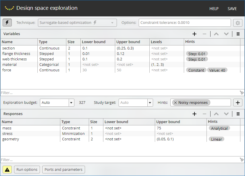
Suppose, for example, that your Design space exploration block has three responses defined with different function types:

• Analytical constraint response mass ("Function type" hint set to Analytical). The response port name is Blackbox.mass.
• Optimization response stress represents a generic objective function ("Function type" hint is missing). The response port name is Blackbox.stress.
• Linear constraint response geometry ("Function type" hint set to Linear). The response port name is Blackbox.geometry.

Suppose that three blocks are used to evaluate the three responses listed above, with the block names matching the response names: the "Mass" block, the "Stress" block, and the "Geometry" block. Let's also assume that each of these three blocks has the section input to receive the values of the section variable, and the response output to issue the values of the corresponding response. Then, to connect the Design space exploration block to the blackboxes in the workflow, you will need to create the following links:

• From the Blackbox.section request port to the section input of each of those three blocks - "Mass", "Stress", and "Geometry".
• From the "Mass" block's response output to the Blackbox.mass response port.
• From the "Stress" block's response output to the Blackbox.stress response port.
• From the "Geometry" block's response output to the Blackbox.geometry response port.

Initial samples

Initial sample is optional input data sent to the block - an existing designs sample that can be used in several ways depending on the block configuration. The initial sample can contain either values of variables, or values of both variables and responses.

The initial sample data is used as follows:

• Non-adaptive design of experiment generation techniques add the generated new designs to the initial sample, and then process the obtained sample according to the current block configuration. For example, if there are constraint responses, all designs are checked for feasibility; if a blackbox is connected, all feasible designs are evaluated, and so on.
• The Initial sample evaluation technique processes the initial sample in the same way, it just does not generate any new design points.
• If the initial sample is a Latin hypercube design, the Latin hypercube sampling technique can update it (generate new designs) in such a way that the new sample is also a Latin hypercube. To enable this special mode, the technique provides the "Property preservation" option.
• Adaptive design of experiment generation techniques can use the initial sample to train initial approximations of the response functions, thus improving generation quality. Another usage pattern is when your configuration includes an adaptive type response that is not evaluated by a blackbox: in this case, the technique requires an initial sample for this response, and uses it to train an internal model that is used to evaluate the response instead of the blackbox.
• The Surrogate-based optimization- technique uses the initial sample to train initial approximation models of responses. If the initial sample does not contain response values, or some of them are missing, these designs are evaluated first.
• The Gradient-based optimization technique uses the initial sample as an extended initial guess. If the initial sample contains both variable and response values, this technique selects optimum designs from the initial sample and starts searching from those points. If response values are missing, the initial designs are evaluated first, and then analyzed for optimality.

The initial sample can be supplied as a single table, as two separate tables with values of variables and responses, or as a number of separate samples - one for each variable and response.

• The Initial sample input accepts the single initial sample table. The order of table columns should follow the order of variables and responses as they are listed in the Variables pane and Responses pane, with variables going first. The response part can be omitted: the number of table columns should either be equal to the total of the variables' "Size" values, or be equal to the total of the variables' "Size" values together with the total of the responses' "Size" values. For a multi-dimensional variable or response, the number of the corresponding table columns is equal to the "Size" value of that variable or response.

• Additional ports that accept initial samples can be enabled in the Ports and parameters dialog (see Ports and parameters):

  • The Variables.Initial sample and Responses.Initial sample ports accept initial values of variables and responses as two separate tables. The number of columns in the table of variables (responses) is equal to the total of the variables' (responses') "Size" values. The table of responses can be omitted - for example, if you do not connect the Responses.Initial sample port, this is interpreted as missing response values. However, if you pass the response data to the Responses.Initial sample input, then you must also send the variable data to the Variables.Initial sample input; in this case, both tables must have the same number of rows.

    The Variables.Initial sample and Responses.Initial sample ports can be useful if you need to pass a full initial sample but its variable and response parts come from different blocks. If you need to pass an initial sample of variables only, just send it to the Initial sample port.

  • You can also enable component-wise initial sample ports. Their names follow the <variable-name>.Initial sample and <response-name>.Initial sample pattern. These ports accept sample table with the number of columns in each table equal to the "Size" of the respective variable or response. All tables sent to component-wise initial sample ports must have the same number of rows. In this case, none of the response component-wise initial samples can be omitted.

    Component-wise sample ports can be useful, for example, should you want to omit initial samples only for some of the responses: all the <response-name>.Initial sample ports are optional, and if any one of them is not connected, this is interpreted as missing values for the respective response. However, if you pass data to any of the <response-name>.Initial sample ports, then all <variable-name>.Initial sample ports must also receive input data. Due to this, in certain cases it might be more convenient to use the Variables.Initial sample and Responses.Initial sample ports, and pass to the Responses.Initial sample input a table that has the corresponding request columns filled with N/A literals, see below.

The input part of the initial sample (variable values) must be fully defined, that is, it cannot contain missing (N/A) or undefined (NaN) values, or empty columns. The output part (response values), however, is allowed to contain special values that have the following meaning:

• The NaN value means that the response cannot be evaluated in the corresponding design point. The block treats such points as infeasible.

• The N/A value means that the response was not evaluated in the corresponding design point.

  The block tests such points for feasibility (evaluating constraints, if they are missing), and then processes feasible initial points in accordance with the current technique - for example, evaluates objectives in the case of an optimization study.

  An empty column can be created in the response part of the initial sample by filling it with N/A values. Note that the column cannot be removed even if it is empty, since this would change the shape of the sample table.

Note that the initial sample is processed in a specific way if there are categorical or discrete variables in the block configuration, and the block runs a technique that does not provide full support for these types of variables (for example, some design of experiment generation techniques). In such cases the block performs a number of independent runs, one for each possible combination of variable levels. The initial sample is split between these runs according to values of variables in each combination, so each run actually uses its own initial sample, which is only a subset of the original. These subsets can contain different number of design points, which can lead to different technique behavior in different runs.

Block operation results

Result ports

Regardless of its configuration, the block always produces 3 result samples, and outputs them as tables on the following ports:

• The All designs port outputs the sample containing all generated data - the design points (variable values) generated by the block and the response values calculated in the blackboxes.

  Note that response values at some points might be missing - this means that the response at the given point has not been calculated. By default, this result sample also includes initial sample points; you can exclude them from the result sample using the Include initial sample option.

• The Feasible designs port outputs the sample containing all feasible points.

  A design point deems feasible if it satisfies the specified constraints, has continuous and stepped variable values within the specified bounds, discrete and categorical variable values match the specified levels, and stepped variable values comply with the specified step settings.

  In certain cases, this sample is the same as the sample issued on the All designs output - for example, when there are no constraint responses in the block configuration, and the initial sample is not used or contains only feasible points. Also, the feasible result set never includes points that are missing any response values.

• The Optimal designs port outputs the sample containing all points that are both feasible and optimal with regard to responses of the minimization/maximization type.

  If the block configuration does not define minimization/maximization responses, the optimal result set is the same as the feasible one.

In most cases, the optimal result set should be considered the main result. In simple design of experiment generation tasks (no constraint responses, no initial sample), the contents of all three result sets are the same: the optimal result contains all generated points. In constrained design of experiment generation tasks without minimization or maximization responses, the optimal and feasible results are the same: the optimal result contains all feasible points. In optimization tasks, the optimal result set provides the solution to the given optimization problem, and so on.

The sample that is output on the All designs port does not exactly represent the evaluation history: it is compacted to reduce the number of missing response values. For example, suppose there are two responses depending on the same variables, but evaluated by different blackboxes. In the evaluation history, each design point evaluated by both blackboxes would create two history entries, and each entry would contain values of all variables but only one response value. In the result sample, these entries are merged to a single table row containing all variable and response values. Due to this, the number of rows in the All designs table is generally not equal to the total number of evaluations performed.

In addition to the ports described above, you can use additional ports that output separate result tables for all variables and all responses, or individual result tables for each variable and each response. For details on those ports, see Ports and parameters.

Feasibility measure

The block can calculate a feasibility measure (constraint violation measure) for each design point in the results, and output this data to the Feasibility.All designs, Feasibility.Feasible designs, and Feasibility.Optimal designs ports (see Ports and parameters for details).

Given a design point $x$, its feasibility measure is defined as $\psi(x) = \max_i \psi_i(x)$, where $\psi_i(x)$ are individual constraint violation measures. The $\psi_i(x)$ values are calculated separately for each constraint $c_i$ with the lower bound $l_i$ and upper bound $u_i$ as follows: $$ \psi_i(x) = \max\left[ \frac{l_i - c_i(x)}{\max(1, |l_i|)}, \frac{c_i(x) - u_i}{\max(1, |u_i|)} \right]. $$ So, $\psi_i(x) > 0$ indicates that the constraint $c_i$ is violated, and $\psi_i(x) \leq 0$ indicates that this constraint is met. Since $\psi(x) = \max_i \psi_i(x)$, it is positive ($\psi(x) > 0$) if $x$ violates at least one of the constraints. The value of $\psi_i(x)$ can also be understood as the normalized distance from the value of the response $c_i$ at the point $x$ to the bounds of that response, negative in the interval between the bounds and positive outside this interval. The feasibility measure $\psi(x)$ is then the maximum of those distances.

Result files

In its working directory, the Design space exploration block creates a subfolder where it stores its results as files. That folder has the same name as the block; if such a folder name happens to be not unique, it is prepended with the name of the parent Composite block. The folder contains:

• Designs.csv, History.csv (only in optimization and adaptive design) - the intermediate result and the raw history of evaluations (see below).
• Results subfolder - the final result files:
  • All designs.csv, All designs.p7table - all collected data, the same as the table output to the All designs port.
  • Feasible designs.csv, Feasible designs.p7table - feasible points only, the same as the table output to the Feasible designs port.
  • Optimal designs.csv, Optimal designs.p7table - optimal points only, the same as the table output to the Optimal designs port.

Intermediate result and evaluation history

Once the Design space exploration block starts, it creates the Designs.csv and History.csv files and begins updating them with variable and response data.

History.csv contains the raw history of evaluations. Each row exactly corresponds to a single evaluation request issued by the Design space exploration block to a certain blackbox block. For example, if there are 2 responses evaluated by different blackboxes, and their values are requested for the same design point, the history contains 2 corresponding rows, as those are 2 separate requests.

Designs.csv is the intermediate result. This table stores design points: following the above example, the 2 evaluations, which appear as separate rows in History.csv, would appear as a single row in Designs.csv, as they actually correspond to a single design point.

The response columns in both History.csv and Designs.csv may contain NaN values (denoted nan) and N/A values (missing values, denoted by empty CSV fields).

Designs.csv contains additional columns with design point classifiers and point description:

• The "feasible" column may contain the following values:
  • 1 - feasible point: all constraints are evaluated, neither constraint is violated or NaN.
  • 0 - infeasible point: at least one constraint is violated or NaN.
  • -1 - feasibility not yet known: for example, some constraints were evaluated and they are satisfied, but there are other constraints that are not yet evaluated.
• The "optimal" column may contain:
  • 1 - the point might be optimal: it is not dominated by any other known feasible point yet.
  • 0 - the point cannot be optimal: it is already dominated by another known feasible point.
• The "initial" column may contain:
  • 1 - marks the points that are present in the initial sample.
  • 0 - new points generated by the block.
• The "description" column contains a brief human-readable description of the design point.

Each of the classifier columns might rarely contain an empty field, if the block was unable to classify a certain design point.

Note

If a point in the intermediate result is deemed feasible, this outcome is final: by definition, a feasible point cannot be re-qualified as infeasible at subsequent iterations.

If a point in the intermediate result is deemed (currently) optimal, this outcome is not final: some future iteration of the study may produce a better point, which will dominate the currently optimal point.

The classifier columns are intended for post-processing, such as plotting the current designs sample to track the progress of study - see the examples below.

Plotting Designs.csv

import pandas as pd
import plotly.subplots as sp
import plotly.graph_objects as go


# Plot each component (variable, response) against the index of iteration.
def plot_iterations(designs, names=None, filename=None):
    mask_feasible = (designs["feasible"] == 1) + (designs["feasible"] == -1)
    mask_optimal = designs["optimal"] == 1
    mask_initial = designs["initial"] == 1

    if names is None:
        names = [
            name
            for name in designs.columns
            if name not in ["initial", "feasible", "optimal", "description"]
        ]

    fig = sp.make_subplots(rows=len(names), cols=1)
    for i, name in enumerate(names):
        # axis label is the component name, that is column title without the prefix
        fig["layout"][f"yaxis{i+1}"]["title"] = name.split(".")[-1]
        # all designs
        fig.add_trace(
            go.Scatter(
                name="all",
                x=designs.index,
                y=designs[name],
                mode="markers+lines",
                marker_color="grey",
                showlegend=i == 0,
                legendgroup="all",
            ),
            row=i + 1,
            col=1,
        )
        # initial sample designs
        fig.add_trace(
            go.Scatter(
                name="initial",
                x=designs[mask_initial].index,
                y=designs[mask_initial][name],
                mode="markers",
                marker_color="black",
                marker_symbol="circle-open",
                marker_size=10,
                showlegend=i == 0,
                legendgroup="initial",
            ),
            row=i + 1,
            col=1,
        )
        # feasible designs
        fig.add_trace(
            go.Scatter(
                name="feasible",
                x=designs[mask_feasible].index,
                y=designs[mask_feasible][name],
                mode="markers",
                marker_color="blue",
                showlegend=i == 0,
                legendgroup="feasible",
            ),
            row=i + 1,
            col=1,
        )
        # optimal designs
        fig.add_trace(
            go.Scatter(
                name="optimal",
                x=designs[mask_optimal].index,
                y=designs[mask_optimal][name],
                mode="markers",
                marker_color="red",
                marker_size=4,
                showlegend=i == 0,
                legendgroup="optimal",
            ),
            row=i + 1,
            col=1,
        )
    fig["layout"][f"xaxis{i+1}"]["title"] = "Iteration"
    fig.update_layout(width=1000, height=800)
    if filename is not None:
        fig.write_html(f"Designs - {filename}.html")
        fig.write_image(f"Designs - {filename}.png")


# Plot each variable-response pair.
def plot_pairwise(designs, x_names=None, y_names=None, filename=None):
    mask_feasible = (designs["feasible"] == 1) + (designs["feasible"] == -1)
    mask_optimal = designs["optimal"] == 1
    mask_initial = designs["initial"] == 1

    if x_names is None:
        x_names = [
            name
            for name in designs.columns
            if name not in ["initial", "feasible", "optimal", "description"]
        ]

    if y_names is None:
        y_names = [
            name
            for name in designs.columns
            if name not in ["initial", "feasible", "optimal", "description"]
        ]

    fig = sp.make_subplots(rows=len(y_names), cols=len(x_names))
    for i, y_name in enumerate(y_names):
        for j, x_name in enumerate(x_names):
            # axis labels are component names - column titles without the prefixes
            fig["layout"][f"xaxis{i*len(x_names)+j+1}"]["title"] = x_name.split(".")[-1]
            fig["layout"][f"yaxis{i*len(x_names)+j+1}"]["title"] = y_name.split(".")[-1]
            # all designs
            fig.add_trace(
                go.Scatter(
                    name="all",
                    x=designs[x_name],
                    y=designs[y_name],
                    mode="markers",
                    marker_color="grey",
                    showlegend=i == j == 0,
                    legendgroup="all",
                ),
                row=i + 1,
                col=j + 1,
            )
            # initial sample designs
            fig.add_trace(
                go.Scatter(
                    name="initial",
                    x=designs[mask_initial][x_name],
                    y=designs[mask_initial][y_name],
                    mode="markers",
                    marker_color="black",
                    marker_symbol="circle-open",
                    marker_size=10,
                    showlegend=i == j == 0,
                    legendgroup="initial",
                ),
                row=i + 1,
                col=j + 1,
            )
            # feasible designs
            fig.add_trace(
                go.Scatter(
                    name="feasible",
                    x=designs[mask_feasible][x_name],
                    y=designs[mask_feasible][y_name],
                    mode="markers",
                    marker_color="blue",
                    showlegend=i == j == 0,
                    legendgroup="feasible",
                ),
                row=i + 1,
                col=j + 1,
            )
            # optimal designs
            fig.add_trace(
                go.Scatter(
                    name="optimal",
                    x=designs[mask_optimal][x_name],
                    y=designs[mask_optimal][y_name],
                    mode="markers",
                    marker_color="red",
                    marker_size=4,
                    showlegend=i == j == 0,
                    legendgroup="optimal",
                ),
                row=i + 1,
                col=j + 1,
            )
    fig.update_layout(width=1000, height=800)
    if filename is not None:
        fig.write_html(f"Designs - {filename}.html")
        fig.write_image(f"Designs - {filename}.png")


# Read the designs table and select the components to plot.
# Note that the interactive HTML plots created by these functions
# are about 3 MB in size.
designs = pd.read_csv("Designs.csv")
plot_iterations(
    designs,
    names=["f.Mass", "c.Stress"],
    filename="history"
)
plot_pairwise(
    designs,
    x_names=["x.r2", "x.r3", "x.r4"],
    y_names=["f.Mass", "c.Stress", "c.g"],
    filename="pairwise",
)

Filtering the N/A (missing) and NaN values

import pyarrow as pa
import pyarrow.csv

options = pa.csv.ConvertOptions(null_values=[""], strings_can_be_null=True)
designs = pa.csv.read_csv("Designs.csv", convert_options=options)

# Get the mask, which is `true` for N/A and `false` for other values.
designs["c.Stress"].is_null()
# Get the mask, which is `true` for NaN values, `null` for N/A, and `false` otherwise.
designs["c.Stress"].is_nan()

Run options

Run options control some features of the block execution and its interaction with other blocks in the workflow:

• Batch mode - enable or disable batch response evaluation mode.
• Detailed log - output detailed information to the workflow run log.
• Deterministic - configures deterministic generation of randomized designs.
• Error handling behavior - the action to perform if the block encounters an error.
• Include initial sample - include points from the initial sample into the result sample.
• Maximum batch size - the maximum number of points that the block may request to evaluate in a single batch when running in batch mode.
• Random seed - seed value for randomized generation algorithms.

Batch mode

Toggles batch response evaluation mode.

• Valid settings: True (enable batch mode), False (disable batch mode)
• Default setting: False (disable batch mode)

Most design space exploration techniques generate new points in batches:

• Space-filling design of experience generation techniques generate the entire sample in one pass.
• Each iteration of the Gradient-based optimization technique requests a batch of evaluations required to estimate response gradients.
• The adaptive design of experiment generation techniques, such as Adaptive design and Adaptive design for GP, and the Surrogate-based optimization technique request batch evaluations when updating internal response models.

If batch mode is enabled, the point batches are output as they are generated by the technique. In that case, request ports output arrays of several elements, where each element of the array represents the variable value at a certain design point and the entire array represents the variable values for all points in the batch. If batch mode is disabled, then the variable values are output through the request ports in the form of numeric scalars or vectors, each of which represents the value of the variable at a single point in the batch.

With the space-filling design of experiment generation techniques and the Gradient-based optimization technique, the number of points in each batch - the batch size - is entirely determined by the task settings and, in the case of optimization, by the currently running stage of the underlying algorithm:

• For space-filling design of experiment generation techniques, the batch size is equal to the size of the generated design of experiment.
• For the Gradient-based optimization technique, the batch size depends on how many gradient estimates are required, which in turn depends on the dimension of the optimization problem - the number of variables, responses, and their dimensions ("Size" property).

At that, you can split the batches generated by the above techniques into a number of smaller batches using the Maximum batch size option - for example, split a space-filling design of experiment to evaluate it in parts.

In the case of adaptive design of experiment generation and Surrogate-based optimization techniques, the batch size also depends on task settings, but can be adjusted when evaluating generic responses, which are considered computationally expensive. By default, those techniques aim to generate batches of minimum possible size when requesting evaluations of generic responses, in order to save computing resources (other response types are considered cheap and can be evaluated in big batches). If the blackbox that evaluates generic responses provides for parallel computing, this default behavior of the technique may lead to inefficient use of computing resources: often, the batch size is not a multiple of the blackbox's parallelization factor meaning that the evaluation of such a batch cannot be efficiently parallelized and some of the batch processors will remain unused because they have no data to process.

To improve the efficiency of parallel computing, it is recommended to set the Maximum batch size option to the maximum parallelization factor specified for the block that implements the blackbox. As a result, the techniques in question switch to an alternative implementation that aims at generating batches, the size of which is a multiple of the Maximum batch size option setting, so they can be evenly split into batches of the specified maximum size when output to the blackbox. This switchover is not performed automatically when enabling batch mode, because the alternative implementation of the study technique differs significantly from the default one, and using it not as intended may cause performance degradation or adversely affect the quality of the block operation results.

Also note that setting the Maximum batch size option in the adaptive design of experiment generation and Surrogate-based optimization techniques does not guarantee that the batch is exactly the specified size, as they are not always able to provide the specified number of points for response evaluation. At some stages of the study, the block may output batches containing fewer points than the option specifies. However, those study techniques tend to minimize the number of such "uneven" batches, thereby increasing the efficiency of parallel evaluations.

In the case of the Gradient-based optimization technique, the Maximum batch size option has no effect on how the technique works, but it indicates that the blackbox being used supports parallel evaluations, and adjusts the effect of the "Exploration budget" setting accordingly.

Regardless of the Batch mode option setting, each of the result samples is always represented as a single table, as described in Block operation results.

Detailed log

Output detailed information to the workflow run log.

• Valid settings: True (enable detailed log), False (disable detailed log)
• Default setting: False (disable detailed log)

Allows the block to white extended debugging information to the run log. Note that enabling this option can result in very large logs.

To view the debugging messages, select the "Show debug" command from the context menu in the Run log pane that displays run logs.

Deterministic

Configures deterministic generation of randomized designs.

• Valid settings: Disable, Block run
• Default setting: Block run

Fix the seed for all randomized design of experiment generation techniques for each run of the block, or disable deterministic behavior. To set the seed, use the Random seed option.

This option affects the following design of experiment generation techniques that use a pseudo-random number sequence:

• Latin hypercube sampling
• Random uniform sequence
• Adaptive design
• Adaptive design for GP
• Orthogonal array design
• D-optimal design
• I-optimal design
• Box-Behnken design

Other techniques do not use a pseudo-random number sequence, so they are always deterministic, and are not affected by this option.

Error handling behavior

The action to perform if the block encounters an error.

• Valid settings: stop workflow, output defaults
• Default setting: stop workflow

When this option is set to stop workflow, the block just reports an error and the workflow run terminates prematurely.

If you set this option to output defaults, the block suppresses the error. In this case, instead of issuing the result samples it has generated, the block outputs the values assigned to its result output ports (the defaults), and the workflow continues to run.

Include initial sample

Include points from the initial sample into the result sample.

• Valid settings: True (include), False (do not include)
• Default setting: True (include)

By default, the points from the initial sample are evaluated and included in the result together with the new generated designs. If this option is set to False, the result samples will contain only the new points. Note that the False setting has no effect on how the block handles initial samples, described in Initial samples.

Maximum batch size

The maximum number of points that the block may request to evaluate in a single batch.

• Valid settings: Auto or an integer from 2 to 512
• Default setting: Auto (allow batches of arbitrary size)

This option is intended to make more efficient use of blackboxes that can run multiple evaluations in parallel, and also can be used to split point batches generated by some techniques into smaller batches, which is important for writing intermediate results.

This option sets the upper limit on the size of the batches of points the block outputs for evaluations, alters the "Exploration budget" setting in the adaptive design and Surrogate-based optimization techniques, and adjusts behavior of those techniques. The non-default option setting should be equal to the blackbox's maximum parallelization factor, that is, the maximum number of parallel calculations the blackbox can run when evaluating responses - for further details, see the Batch mode option description.

For the space-filling design of experiment techniques, this option does not affect the technique behavior (the DoE it generates), though can be used to split the DoE into batches of the specified size. The sole exception is the final batch in the case when the DoE size (the "Exploration budget" setting) is not a multiple of the option value - obviously, the final batch gets the remainder of points. The "Exploration budget" setting always specifies the total number of generated points (the final DoE size), in batch mode as well, regardless of the Maximum batch size setting.

For the optimization and adaptive design techniques in batch mode, if the Maximum batch size option is set to a certain numerical value p, the "Exploration budget" setting specifies the limit for the total number of batches the block outputs for evaluation, with each of those batches containing at most p design points. Thus, the "Exploration budget" setting limits the number of batch evaluation requests the block can send to the blackbox, rather than the total number of points in those requests.

In the case of the Gradient-based optimization technique, the Maximum batch size option only affects the "Exploration budget" setting as described above, and has no effect on the optimization technique itself. As for the adaptive design of experiment generation and Surrogate-based optimization techniques, this option also adjusts the behavior of the technique so that the total batch it generates can be evenly split into batches of the specified maximum size. This adjustment only affects the batches that request evaluation of generic responses, which are computationally expensive; batches related to computationally cheap responses may be of arbitrary size.

Note that setting the Maximum batch size option does not guarantee that the batch is exactly the specified size, as the study technique is not always able to provide the specified number of points for evaluation. At some stages of the study, the block may output batches containing fewer points than the option specifies. However, the adaptive design of experiment generation and Surrogate-based optimization techniques tend to minimize the number of such "uneven" batches, thereby increasing the efficiency of parallel evaluations.

With the abovementioned techniques, the Maximum batch size option affects the operation of the block, significantly changing the technique behavior. Therefore, it should only be set if the block that serves as the blackbox is indeed capable of parallel computing, that is, it can synchronously perform two or more evaluations, each using an independent processing unit with dedicated resources. Failure to comply with this condition may adversely affect the technique performance or the quality of its results. If you use an adaptive design of experiments technique or Surrogate-based optimization, and enable batch mode with the Batch mode option, but the blackbox only provides sequential processing of batch points, then the Maximum batch size option should be left at the default setting (Auto), and the blackbox implementation must be able to handle batches of arbitrary size.

Random seed

Seed value for randomized generation algorithms.

• Valid settings: a positive integer
• Default setting: 100

The value of this option is used to seed all randomized generation methods when deterministic generation is enabled with the Deterministic option. If deterministic generation is disabled, the Random seed option has no effect.